Microsoft 365 Training


Are you a small business?
Visit the small business help & learning page to learn how you can use Microsoft 365 in your small business.

Collaborate
Do your best work together. With Microsoft 365, you can collaborate with anyone, anywhere.
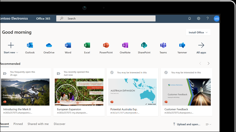
Microsoft 365 for the web training
Learn how to stay productive in Microsoft 365 from any browser with these brand new courses.


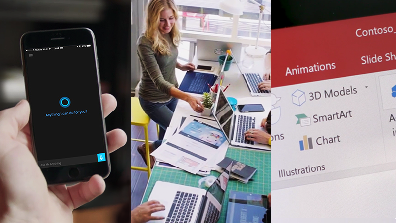
Modern workplace training
Learn how to get more work done, from anywhere on any device with Microsoft 365 and Windows 10. Discover how industry professionals leverage Microsoft 365 to communicate, collaborate, and improve productivity across the team and organization.